Introduction
In my last semester of college, I took a course in non-linear dynamics and chaos theory as part of a minor in mathematics that I earned at the University of Michigan. As part of the course, the final project was to take the principles learned in modeling dynamic systems and apply them to an interesting scenario. A fellow classmate and I decided (as we were both engineers) to try to model the dynamics of the following theoretical system. For the full report we wrote, click here. Here, I will cover an abbreviated version. If you just want to see the videos/simulations, scroll all the way down.
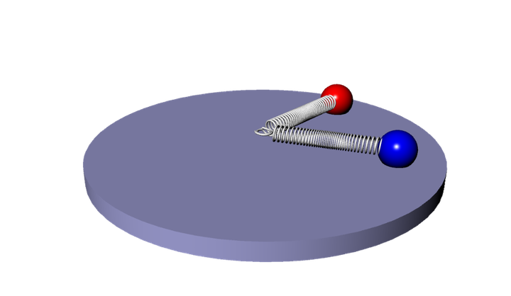
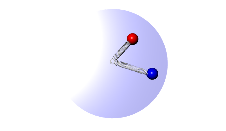
The system we derived and wanted to understand is a system of two charged masses each attached to a center point by a spring (see figures below). We will explain how we derived this system from basic physics principles and how we tested our model to make sure it did not exhibit unrealistic behaviors. We then analyze the system by first changing the dimensional system into a dimensionless one. We do this because a dimensionless system makes our analysis simpler by looking at the ratios of parameters (more on this later). Finally, we find the fixed points, attempt to characterize them, and understand when the system becomes choatic. The challenge turned out harder than we expected but the effort was rewarding.

Governing Physics Equations
Translational Accelerations
![]()
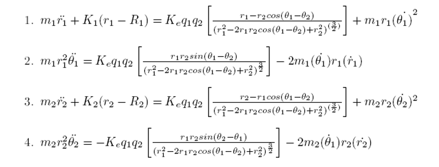
These equations reflect the idea that the sum of the forces in the radial direction on both masses will dictate the radial acceleration of the masses. Since the forces of the spring and centripetal motion are always in the radial direction, these forces are always purely in these directions. However, since the electric force depends on the relative location of the masses, the radial force must be calculated calculating the component of the electric force that is along the radial direction.
Rotational Accelerations
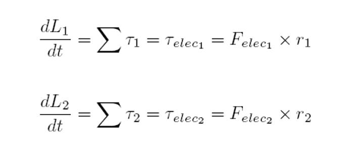
These equations reflect the idea that the change in angular momentum is equivalent to the sum of the torques on the individual masses. Since the only possible torque in the system can come from the electric field, it is the only component we account for in these equations. We can also see that the torque is calculated as the cross product between the electric force and the lever arm that is the length of r.
Governing Differential Equations
These equations can be written in the form of 4 coupled 2nd-order differential equations as follows:
The above equations can then be re-written in the form of a 8 first-order differential equations as follows:
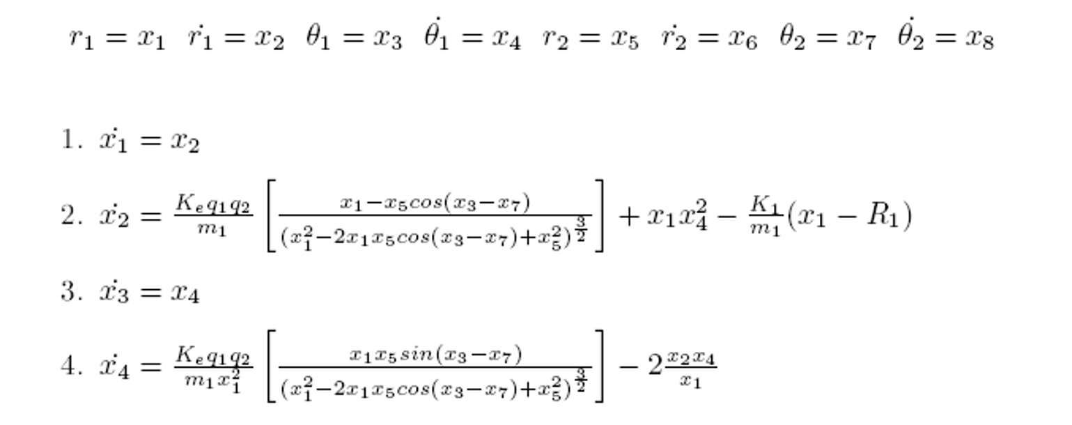
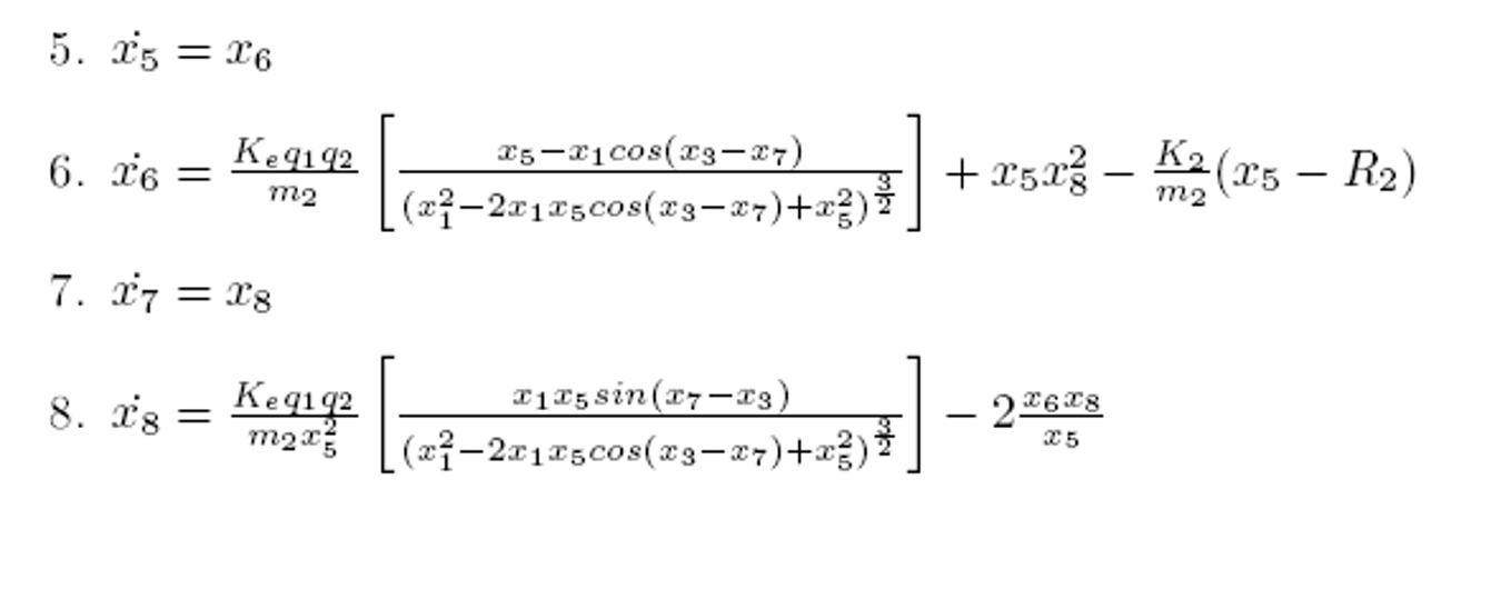
I will leave the proofs and further analysis in the report for those who are interested. There is some pretty interesting nuances in modeling this dynamic system in ways that obey physical laws. But below, I’ll show some interesting results from simulations of this dynamic system.
Simulations
First, we start with a simple system of these two masses with no electrical charge in the system. We set their initial radial/angular positions and velocities and can watch the dynamics.
Next, we can set the charges to positive values to simulate two positively charged masses that should repel each other.
Finally, we show an interesting simulation where one particle starts with only radial velocity and the other one begins with both radial and angular velocity. Additionally, these particles are oppositely charged so they will attract each other.
Link to the code on github here. You can run the main.m file as main(time,plot_type,range,filename) and change the following parameters:
- time = 100 (time to run sim)
- plot_type = 2 (set to 2 to make video)
- range = 1 (deprecated)
- filename = filename for video
system parameters in Testfunction.m
% K1,K2 = spring constants
% q1,q2 = charge values
% m1,m2 = mass of particles
% R1,R2 = length of springs

function [dx_dt]=Testfunction(t,x);
K1=10; K2=10; q1=0; q2=0; m1=1; m2=1;R1=1;R2=1;Ke= 8.987e9;
initial conditions in main.m
% radial position - particle1, radial velocity - particle1, angular position - particle1, angular velocity - particle1
% radial position - particle2, radial velocity - particle2, angular position - particle2, angular velocity - particle2

function main(tim,ch,range,filename);
Xo=[1;1;pi;0.5;1;1;0;-.5];